Vignette
This vignette extends the vignette for the R-version of tximport. If you are unfamiliar with tximport or curious about the motivation behind it, please check it out.
If you are looking for a full-featured end-to-end workflow for Pythonic bulk RNA-sequencing analysis, check out our Snakemake workflow based on pytximport.
Creating your transcript to gene map
Here, we will show you how to generate a transcript-to-gene mapping based on the Ensembl reference or a gene transfer format file.
Build it from Ensembl
This example requires pybiomart which is installed together with pytximport. Providing a host is optional, for a list of available archives that correspond to Ensembl releases, please consult https://www.ensembl.org/info/website/archives/index.html. By default, the transcript ids will be mapped to the ensembl_gene_id field. If you prefer to use gene names, choose external_gene_name. Be aware that not all proposed transcripts have been assigned a name yet and thus will not be
included if you use gene names. The first time you run this function, it may take a few seconds to download the data.
[1]:
from pytximport.utils import create_transcript_gene_map

transcript_gene_map_human = create_transcript_gene_map(
    species="human",
    target_field="external_gene_name",
)
transcript_gene_map_human.head(5)
[1]:
| transcript_id | gene_id | |
|---|---|---|
| 0 | ENST00000387314 | MT-TF |
| 1 | ENST00000389680 | MT-RNR1 |
| 2 | ENST00000387342 | MT-TV |
| 3 | ENST00000387347 | MT-RNR2 |
| 4 | ENST00000386347 | MT-TL1 |
[2]:
transcript_gene_map_mouse = create_transcript_gene_map(species="mouse")
transcript_gene_map_mouse.head(5)
[2]:
| transcript_id | gene_id | |
|---|---|---|
| 0 | ENSMUST00000082387 | ENSMUSG00000064336 |
| 1 | ENSMUST00000082388 | ENSMUSG00000064337 |
| 2 | ENSMUST00000082389 | ENSMUSG00000064338 |
| 3 | ENSMUST00000082390 | ENSMUSG00000064339 |
| 4 | ENSMUST00000082391 | ENSMUSG00000064340 |
You can also provide a list of mapping targets as the target_field argument. For example, to map transcripts to both gene names and gene biotypes, you can use the following code:
[3]:
transcript_gene_map_human_biotype = create_transcript_gene_map(
    species="human",
    target_field=["external_gene_name", "gene_biotype"],
)
transcript_gene_map_human_biotype = transcript_gene_map_human_biotype[
    transcript_gene_map_human_biotype["gene_biotype"] == "lncRNA"
]
transcript_gene_map_human_biotype.head(5)
[3]:
| transcript_id | gene_id | gene_biotype | |
|---|---|---|---|
| 94 | ENST00000632454 | LINC01784 | lncRNA |
| 118 | ENST00000707308 | LINC02688 | lncRNA |
| 119 | ENST00000707309 | LINC02688 | lncRNA |
| 164 | ENST00000631340 | LINC02735 | lncRNA |
| 181 | ENST00000672718 | AGAP12P | lncRNA |
Use a gene transfer format file
If you already have an annotation file in .gtf format (e.g. from the GENCODE or Ensembl references), you can use the create_transcript_gene_map_from_annotation function contained in pytximport.utils to generate a transcript to gene map. Using an annotation file is considered best practice, as it ensures that your annotation and alignment reference are the same if you download them from the same source, e.g., an Ensembl release.
Set target_field to gene_name to map transcript ids to gene names instead of gene ids. If the transcript does not have a corresponding gene name in the annotation file, it will be mapped to the gene id.
[4]:
from pytximport.utils import create_transcript_gene_map_from_annotation

transcript_gene_map_from_gtf = create_transcript_gene_map_from_annotation(
    "../../test/data/annotation.gtf",
    target_field="gene_name",
)
transcript_gene_map_from_gtf.head(5)
[4]:
| transcript_id | gene_id | |
|---|---|---|
| 0 | ENST00000424215 | ENSG00000228037 |
| 1 | ENST00000511072 | PRDM16 |
| 2 | ENST00000607632 | PRDM16 |
| 3 | ENST00000378391 | PRDM16 |
| 4 | ENST00000514189 | PRDM16 |
Map transcript names to gene names
You can also optionally map transcript names to either gene names or gene ids if your data requires it.
[5]:
transcript_name_gene_map_human = create_transcript_gene_map(
    "human",
    source_field="external_transcript_name",
    target_field="external_gene_name",
)
transcript_name_gene_map_human.head(5)
[5]:
| transcript_name | gene_id | |
|---|---|---|
| 0 | MT-TF-201 | MT-TF |
| 1 | MT-RNR1-201 | MT-RNR1 |
| 2 | MT-TV-201 | MT-TV |
| 3 | MT-RNR2-201 | MT-RNR2 |
| 4 | MT-TL1-201 | MT-TL1 |
Importing transcript quantification files
You can easily import quantification files from tools like salmon with pytximport.
[6]:
import numpy as np
import pandas as pd

from pytximport import tximport
[7]:
txi = tximport(
    [
        "../../test/data/salmon/multiple/Sample_1.sf",
        "../../test/data/salmon/multiple/Sample_2.sf",
    ],
    "salmon",
    transcript_gene_map_mouse,
    counts_from_abundance="length_scaled_tpm",
    output_type="xarray",  # or "anndata"
)
txi
Reading quantification files: 2it [00:00, 101.58it/s]
[7]:
<xarray.Dataset> Size: 28kB
Dimensions:    (gene_id: 496, file: 2, file_path: 2)
Coordinates:
  * gene_id    (gene_id) object 4kB 'ENSMUSG00000083355' ... 'ENSMUSG00000067...
  * file_path  (file_path) <U43 344B '../../test/data/salmon/multiple/Sample_...
Dimensions without coordinates: file
Data variables:
    abundance  (gene_id, file) float64 8kB 0.08291 0.0 0.09854 ... 0.4618 0.0
    counts     (gene_id, file) float64 8kB 1.005 0.0 1.086 ... 1.957 6.208 0.0
length (gene_id, file) float64 8kB 509.1 509.1 445.8 ... 564.6 564.6Exporting transcript-level count estimates
You can also export the transformed transcript counts directly for transcript-level analysis.
[8]:
txi = tximport(
    ["../../test/data/salmon/quant.sf"],
    "salmon",
    counts_from_abundance="scaled_tpm",
    return_transcript_data=True,
)
txi
Reading quantification files: 1it [00:00, 207.47it/s]
[8]:
AnnData object with n_obs × n_vars = 1 × 14
    uns: 'counts_from_abundance'
    obsm: 'length', 'abundance'
Note that the example above works without a transcript to gene map. If you want to use the transcript names instead of the transcript ids, you can optionally use the replace_transcript_ids_with_names function together with a transcript id to transcript name map. We can use the create_transcript_gene_map function to create a map between transcript ids and transcript names, too.
[9]:
from pytximport.utils import replace_transcript_ids_with_names
[10]:
transcript_name_map_human = create_transcript_gene_map("human", target_field="external_transcript_name")
transcript_name_map_human.head(5)
[10]:
| transcript_id | transcript_name | |
|---|---|---|
| 0 | ENST00000387314 | MT-TF-201 |
| 1 | ENST00000389680 | MT-RNR1-201 |
| 2 | ENST00000387342 | MT-TV-201 |
| 3 | ENST00000387347 | MT-RNR2-201 |
| 4 | ENST00000386347 | MT-TL1-201 |
[11]:
txi = replace_transcript_ids_with_names(txi, transcript_name_map_human)
pd.DataFrame(txi.X.T, index=txi.var.index, columns=txi.obs.index).sort_values(
    by=txi.obs.index[0],
    ascending=False,
).head(5)
[11]:
| ../../test/data/salmon/quant.sf | |
|---|---|
| HOXC8-201 | 4486.940412 |
| UGT3A2-201 | 1307.314695 |
| HOXC9-201 | 886.909534 |
| HOXC4-202 | 749.069369 |
| HOXC12-201 | 544.817685 |
The same data summarized to genes:
[12]:
txi = tximport(
    ["../../test/data/salmon/quant.sf"],
    "salmon",
    transcript_gene_map_human,
    counts_from_abundance="scaled_tpm",
    output_type="xarray",
    return_transcript_data=False,
)
pd.DataFrame(txi["counts"], index=txi.coords["gene_id"], columns=txi.coords["file_path"]).sort_values(
    by=txi.coords["file_path"].data[0],
    ascending=False,
).head(5)
Reading quantification files: 1it [00:00, 231.92it/s]
[12]:
| ../../test/data/salmon/quant.sf | |
|---|---|
| HOXC8 | 4486.940412 |
| UGT3A2 | 1506.597257 |
| HOXC4 | 1152.964133 |
| HOXC9 | 886.909534 |
| HOXC12 | 544.817685 |
Note that the top transcript corresponds to the top expressed gene in this case.
Exporting AnnData files
pytximport integrates well with other packages from the scverse through its AnnData export option.
[13]:
txi_ad = tximport(
    ["../../test/data/salmon/quant.sf"],
    "salmon",
    transcript_gene_map_human,
    output_type="anndata",
    # the output can optionally be saved to a file by uncommenting the following lines
    # output_format="h5ad",
    # output_path="txi_ad.h5ad",
)
txi_ad
Reading quantification files: 1it [00:00, 309.11it/s]
[13]:
AnnData object with n_obs × n_vars = 1 × 10
    uns: 'counts_from_abundance'
    obsm: 'length', 'abundance'
Exporting SummarizedExperiment files
Experiment support for SummarizedExperiment files is available through the BiocPy ecosystem (unaffiliated). While not part of the core functionality of pytximport, this output type/format may be useful for interacting with other R software packages. The optional dependencies necessary to support SummarizedExperiment files can be installed via pip install pytximport[biocpy].
[14]:
txi_se = tximport(
    ["../../test/data/salmon/quant.sf"],
    "salmon",
    transcript_gene_map_human,
    output_type="summarizedexperiment",
    # the output can optionally be saved to disk by uncommenting the following lines
    # output_format="summarizedexperiment",
    # output_path="txi_se",
)
txi_se.assay_names, txi_se.get_row_names(), txi_se.get_column_names()
Reading quantification files: 1it [00:00, 291.19it/s]
WARNING:root:Support for the SummarizedExperiment output type is experimental.
[14]:
(['counts'],
 Names(['UGT3A2', 'HOXC6', 'HOXC9', 'HOXC11', 'HOXC4', 'HOXC10', 'HOXC13', 'HOXC5', 'HOXC8', 'HOXC12']),
 Names(['../../test/data/salmon/quant.sf']))
Use from the command line
You can run pytximport from the command line, too. Available options can be viewed via the pytximport --help command.
[15]:
!pytximport -i ../../test/data/salmon/quant.sf -t "salmon" -m ../../test/data/gencode.v46.metadata.HGNC.tsv -of "h5ad" -ow -o ../../test/data/salmon/quant.h5ad
2025-10-23 23:53:31,869: Starting the import.
Reading quantification files: 1it [00:00, 65.95it/s]
2025-10-23 23:53:32,208: Converting transcript-level expression to gene-level expression.
2025-10-23 23:53:32,269: Matching gene_ids.
2025-10-23 23:53:32,298: Creating gene abundance.
2025-10-23 23:53:32,520: Creating gene counts.
2025-10-23 23:53:32,520: Creating lengths.
2025-10-23 23:53:32,521: Replacing missing lengths.
2025-10-23 23:53:32,528: Creating gene expression dataset.
2025-10-23 23:53:32,530: Saving the gene-level expression to: ../../test/data/salmon/quant.h5ad.
2025-10-23 23:53:32,539: Finished the import in 0.67 seconds.
You can also create a transcript-to-gene mapping via the pytximport create-map command.
[16]:
!pytximport create-map -i ../../test/data/annotation.gtf -o ./transcript_gene_map.tsv -ow
2025-10-23 23:53:33,997: Creating a transcript-to-gene mapping file.
2025-10-23 23:53:34,009: Created the transcript-to-gene mapping file. Saving the file...
2025-10-23 23:53:34,012: Saved the transcript-to-gene mapping file to ./transcript_gene_map.tsv.
Inferential replicates
pytximport can handle bootstraping replicates provided by salmon and kallisto. When inferential_replicate_transformer is set, the provided function is used to recalculate the counts and abundances for each sample based on the bootstraps.
[17]:
result = tximport(
    [
        "../../test/data/fabry_disease/SRR16504309_wt/",
        "../../test/data/fabry_disease/SRR16504310_wt/",
        "../../test/data/fabry_disease/SRR16504311_ko/",
        "../../test/data/fabry_disease/SRR16504312_ko/",
    ],
    "salmon",
    transcript_gene_map_human,
    inferential_replicates=True,
    inferential_replicate_variance=True,  # whether to calculate the variance of the inferential replicates
    inferential_replicate_transformer=lambda x: np.median(x, axis=1),
    counts_from_abundance="length_scaled_tpm",
)
result
Reading quantification files: 4it [00:01,  2.11it/s]
WARNING:root:Not all transcripts are present in the mapping. 29618 out of 253181 missing. Removing the missing transcripts.
[17]:
AnnData object with n_obs × n_vars = 4 × 41127
    uns: 'counts_from_abundance', 'inferential_replicates'
    obsm: 'length', 'abundance', 'variance'
Biotype filtering
For some use cases, it may be of interest to restrict the results to certain gene_biotypes, e.g., protein-coding only. First, generate a transcript-to-gene mapping from an annotation GTF file that includes the gene biotype.
[18]:
transcript_gene_map_from_gtf_with_biotype = create_transcript_gene_map_from_annotation(
    "../../test/data/annotation.gtf",
    target_field=["gene_name", "gene_biotype"],
)
transcript_gene_map_from_gtf_with_biotype.head(5)
[18]:
| transcript_id | gene_id | gene_biotype | |
|---|---|---|---|
| 0 | ENST00000424215 | ENSG00000228037 | lncRNA |
| 1 | ENST00000511072 | PRDM16 | protein_coding |
| 2 | ENST00000607632 | PRDM16 | protein_coding |
| 3 | ENST00000378391 | PRDM16 | protein_coding |
| 4 | ENST00000514189 | PRDM16 | protein_coding |
Then, import quantification files using the transcript-to-gene mapping and filter the counts by biotype.
[19]:
from pytximport.utils import filter_by_biotype

result_small = tximport(
    ["../../test/data/fabry_disease/SRR16504309_wt/"],
    "salmon",
    transcript_gene_map_from_gtf_with_biotype,
    counts_from_abundance="length_scaled_tpm",
)

result_small_filtered = filter_by_biotype(
    result_small,
    transcript_gene_map_from_gtf_with_biotype,
    biotype_filter=["protein_coding"],
    # Since the data is already at the gene level, we have to use the gene_id from the transcript_gene_map
    id_column="gene_id",
)

len(result_small.var_names), len(result_small_filtered.var_names)
Reading quantification files: 1it [00:00,  2.60it/s]
WARNING:root:Not all transcripts are present in the mapping. 253161 out of 253181 missing. Removing the missing transcripts.
[19]:
(12, 4)
Downstream analysis with PyDESeq2
The output from pytximport can easily be used for downstream analysis with PyDESeq2. For more information on PyDESeq2, please consult its documentation.
[20]:
import decoupler as dc
from pydeseq2.dds import DeseqDataSet
from pydeseq2.default_inference import DefaultInference
from pydeseq2.ds import DeseqStats
/Users/malte/pytximport/.venv/lib/python3.13/site-packages/tqdm/auto.py:21: TqdmWarning: IProgress not found. Please update jupyter and ipywidgets. See https://ipywidgets.readthedocs.io/en/stable/user_install.html
  from .autonotebook import tqdm as notebook_tqdm
Load the .csv file generated by pytximport via the output_path argument or create it directly from the output of pytximport. In this case, we are working with the salmon quantification files from a public bulk RNA sequencing dataset: Podocyte injury in Fabry nephropathy
Round count estimates (required by PyDESeq2) and add the corresponding metadata.
[21]:
result.X = result.X.round().astype(int)
result.obs["condition"] = ["Control", "Control", "Disease", "Disease"]
result
[21]:
AnnData object with n_obs × n_vars = 4 × 41127
    obs: 'condition'
    uns: 'counts_from_abundance', 'inferential_replicates'
    obsm: 'length', 'abundance', 'variance'
Filter genes with low counts out.
[22]:
result = result[:, result.X.max(axis=0) > 10].copy()
result
[22]:
AnnData object with n_obs × n_vars = 4 × 14776
    obs: 'condition'
    uns: 'counts_from_abundance', 'inferential_replicates'
    obsm: 'length', 'abundance', 'variance'
Now perform your PyDESeq2 analysis.
[23]:
dds = DeseqDataSet(
    adata=result,
    design="~condition",
    refit_cooks=True,
    inference=DefaultInference(n_cpus=8),
    quiet=True,
)
[24]:
dds.deseq2()
/Users/malte/pytximport/.venv/lib/python3.13/site-packages/pydeseq2/dds.py:541: UserWarning: As the residual degrees of freedom is less than 3, the distribution of log dispersions is especially asymmetric and likely to be poorly estimated by the MAD.
  self.fit_dispersion_prior()
[25]:
stat_result = DeseqStats(dds, contrast=["condition", "Disease", "Control"], quiet=True)
[26]:
stat_result.summary()
stat_result.lfc_shrink(coeff="condition[T.Disease]")
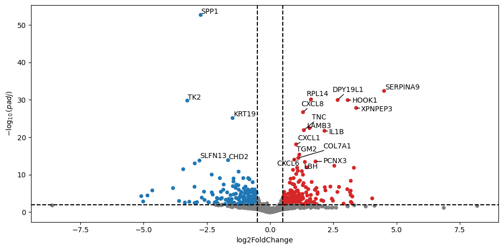
[27]:
dc.pl.volcano(
    stat_result.results_df,
    x="log2FoldChange",
    y="padj",
    thr_sign=0.01,
    top=20,
    figsize=(10, 5),
)
[28]:
collectri = dc.op.collectri(organism="human", remove_complexes=False)
data = stat_result.results_df[["stat"]].T.rename(index={"stat": "disease.vs.control"})
tf_acts, tf_pvals = dc.mt.ulm(data=data, net=collectri, tmin=5)
dc.pl.barplot(data=tf_acts, name="disease.vs.control", top=10, vertical=True, figsize=(5, 3))

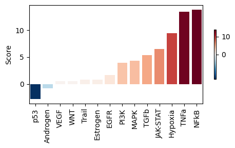
We can also evaluate known pathways.
[29]:
progeny = dc.op.progeny(organism="human", top=500)
pathway_acts, pathway_pvals = dc.mt.ulm(data=data, net=progeny, tmin=5)
[30]:
dc.pl.barplot(
    data=pathway_acts,
    name="disease.vs.control",
    top=40,
    vertical=True,
    figsize=(5, 3),
)
Please refer to the PyDESeq2 and the decoupler documentation for additional analyses.